By George Whicheloe – Man GLG: How can a quantitative framework help discretionary portfolio managers mitigate behavioural biases?
A common pitfall in investing is cutting winning positions and clinging to losing ones.
Introduction
“Run your winners and cut your losers.”
This principle is, unfortunately, ignored by most portfolio managers. Indeed, a common pitfall in investing is cutting winning positions and clinging to losing ones. Known as the disposition effect, this paradoxical behaviour can be traced back to Kahneman and Tversky’s prospect theory (1979), which posits that the pain of losing is experienced more intensely than the joy of an equivalent gain. This asymmetry can result in portfolio managers demonstrating a risk-seeking attitude towards losses and a risk-averse approach towards unrealised gains.
This is just one example of biases portfolio managers can have. Overconfidence bias, herding bias, and recency bias are others, all of which can strategically influence decision-making.
So how can these influences be mitigated? We previously examined how a quantitative process can discern the true ‘skill’ of portfolio managers by eliminating the noise often associated with the discretionary investment process. The primary objective of the skill measurement framework we developed was to provide timely and tangible feedback to portfolio managers, thereby fostering a more stable environment which would be more conducive to portfolio managers developing skill.
As we rolled out this framework to our portfolio managers, we gained first-hand insights into both effective and ineffective behaviours observed in real-world conditions. After observing these behaviours in action and drawing on behavioural science, we began to propose behavioural changes to managers. In this article, we share some of our findings from this process.
Formulating Effective Recommendations: A Practical Approach
A recommendation is formulated through several potential pathways:
- Sometimes, it’s straightforward: the portfolio manager acknowledges susceptibility to a particular behaviour.
- At other times, a portfolio manager’s investment style is naturally inclined towards a certain behaviour. For instance, a Value manager might tend to exit winning positions prematurely.
- Occasionally, multiple analytics converge on a similar conclusion. For example, if high conviction and low conviction positions are providing similar returns, and if a risk-parity version of the portfolio is outperforming the actual portfolio. In such cases, the recommendation usually leans towards minimising the emphasis on sizing decisions and transitioning towards a more balanced portfolio.
The quantitative framework is there to aid the discretionary manager, not to overrule them.
It’s important that the seed of the recommendation chimes true with the manager. For example, if the manager has a firm belief that the analytics are being distorted by a particular market effect, then the recommendations are more likely to be discounted. In the end, the quantitative framework is there to aid the discretionary manager, not to overrule them.
We note that when we make recommendations to portfolio managers, we are similarly making a call on an uncertain future outcome and that us quants are subject to the same biases that portfolio managers are. However, being aware of our biases can go some way towards mitigating them. The below two biases can be particularly potent when examining a set of behavioural analytics and therefore should be held in mind as we next consider how to measure the impact of recommendations.
- Confirmation bias – searching for confirmatory evidence of a prior held belief.
- Extrapolation bias – expecting a repeat or continuation of past events.
Measuring the Impact of Recommendations
Ensuring the success of any process hinges on effectively measuring the impact, and this also holds true for these recommendations.
To measure this impact, we use a straightforward approach, looking at:
- The level of adherence to the recommendation.
- The difference in performance between a simulation of complete adherence and the actual realised performance.
The recommendations generally adhere to the ‘first do no harm’ principle.
In other words, does the portfolio manager follow through with the recommendation? And was it a good recommendation in the first place?
In a scenario in which the manager wholeheartedly embraces the recommendation, there would, of course, be no difference between the simulated portfolio and actual performance.
It seems tempting to examine the ‘counter-counter factual’ where we simulate the portfolio manager’s previously unproductive behaviour, but this turns out to be fraught with assumptions about that behaviour, so we refrain.
What is important to note here is that the recommendations generally adhere to the ‘first do no harm’ principle. For example, if a manager generally only holds high-conviction positions, we will refrain from advising them to ratchet up the concentration, even if their very highest conviction positions have the highest return.
There is an important by-product of this approach in that recommendations must be algorithmically implementable. For example, rather than saying “hold onto your winners longer”, the framework must decide up front how much longer and how to deal with the impact on the rest of the portfolio if there is another stock in play. Let’s now examine some case studies to see how this operates in practice.
Case Study 1: Mechanical Stop Loss Rule
Assume a manager wants to develop a mechanical stop loss rule to short-circuit the cognitive biases that lead to running losers. Figure 1 shows the level of adherence to the stop loss rule, measured by the amount of gross weight triggered by the rule (dark blue line). The amount triggered peaks in early 2020 during the market turmoil caused by the emergence of Covid. The black vertical dashed line marks the point where the manager started receiving stop loss trigger alerts by the quantitative framework.
We make two observations:
1. Even before the official start of the recommendation, the portfolio manager started to be stricter with losing positions.
2. The percentage of gross underwater continues to decline right up to recent history.
As such, we can confidently say that the manager was on board with the recommendation. However, adherence was not 100%, which would be represented by the percentage of gross underwater hitting zero, so the manager was still employing some discretion.
Note that even though the manager was alerted to any drawdowns exceeding their pre-defined threshold, it was still down to their discretion to divest the position. As we have said before, the quantitative framework is there to aid the discretionary manager, not to overrule them! In this case, the manager may have been aware that divesting immediately has an unconditional positive expected return, but there may be extenuating circumstances that meant it remained prudent to stay in the position.
Figure 2 shows the actual profit and loss (P&L), illustrated by the dark blue line, versus the counterfactual P&L of implementing the mechanical stop loss (yellow line). By the official start of the rule, again marked by the vertical black dashed line, the actual P&L had almost caught up to the counterfactual P&L.
The counterfactual went on to outperform, implying that the mechanical stop loss was the right course of action.
Again, we make two observations:
1. The counterfactual P&L was smoother than the actual P&L.
2. There is a downside to a mechanical stop loss rule, which is stopping positions that would have gone on to be profitable.
Post rule implementation, the counterfactual P&L was reset back to the actual P&L, to determine the distinction between the in-sample period (to the left of the black line) and the out-of-sample period (the right of the black line).
In this case, the portfolio manager did not perfectly mimic the stop loss trigger. As such, the counterfactual went on to outperform, implying that the mechanical stop loss was the right course of action.
Figure 1. Percent of Gross Triggered by Drawdown Rule
Figure 2. Actual P&L Versus Counterfactual P&L
Case Study 2: Greedy In / Patient Out
Assume a manager believes that much of the alpha generated comes from the early stages of new ideas, and that they were leaving money on the table by not getting to full size quickly enough.
Of course, when thinking about alpha versus trading, there must be a consideration of trading costs: the faster the trade, the more costly it is, eating into the alpha. In this case, we looked at scaling into a position over many days, even weeks, in highly liquid names.
To test the manager’s hypothesis, we first looked at entry and exit traces. These traces compute the average stock return before and after the entry into the position (Figure 3) and before and after the exit (Figure 4). There are a few things to note:
1. The stock return appears to be steepest immediately after entry.
2. On entry, the alpha appears to plateau after approximately 100 days.
3. After exiting the position, the stock doesn’t go against the manager, suggesting there would be little harm in holding on for longer.
Figure 3. Entry Trace
Figure 4. Exit Trace
Second, two transformations are introduced in the manager’s portfolio: a greedier entry and a more patient exit.
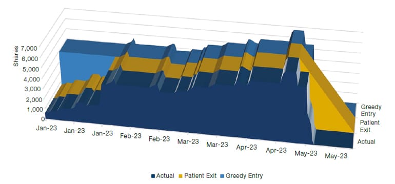
Figure 5 illustrates an example profile of the quantity of shares for one of the manager’s ideas. The actual position (depicted by the dark blue line) is characterised by a rather gentle entry over the first month, which continues to grow until May before being liquidated over a few days.
The first counterfactual simulates the patient exit (depicted by the yellow line), following the original entry, but exiting the position in a more gentle and linear fashion.
The second counterfactual simulates a greedier entry (depicted by the light blue line), hitting the maximum position seen in the first month of the idea and then following the original profile.
Figure 5. Greedy Entry Versus Patient Exit
It’s worth remembering here that it’s not just the relative performance of the counterfactuals that is of interest, but also the level of adherence to the recommendation. Measuring the level of greediness and patience requires creativity. To that end, we define greediness as the area covered by the actual entry versus the greedy entry. We define a similar measure for patience.
To smooth the data, both greediness and patience are measured on a rolling average basis.
As the official start date approached, the greediness measure rose (Figure 6). Intuitively, that makes sense: the idea had been forming in the manager’s mind for some time. Figure 7 illustrates that the counterfactual of 100% greediness significantly outperformed the actual P&L, in both the in-sample and out-of-sample periods. Results from the patience hypothesis, on the other hand, were starkly different: the counterfactual of 100% patience on exit significantly underperformed the actual P&L.
Figure 6. Greediness on Entry
Figure 7. Counterfactual Versus Actual P&L
Figure 8. Patience on Exit
Figure 9. Counterfactual Versus Actual P&L
In a nutshell, greediness on entry worked, but patience on exit didn’t.
In a nutshell, greediness on entry worked, but patience on exit didn’t. Why did this artificial interference with the selling process do such harm to the portfolio?
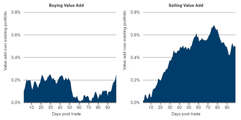
To answer that, we measured the buying and selling skill of the manager. Figure 10 shows the ‘value add’ of adding and reducing positions over a 100-day horizon. What is noteworthy is that the manager is particularly good at selling i.e. being able to identify which idea has run out of steam and quickly ejecting it from the portfolio.
Figure 10. Buying and selling skill
Conclusion
We previously looked at how a quantitative process could discern the true ‘skill’ of a portfolio manager by eliminating the noise associated with the discretionary investment process. The primary objective of the framework was to provide timely and tangible feedback to portfolio managers, fostering an environment conducive to skill development. As a natural next step, we looked at the value of this feedback and have shared some of our findings in this paper.
Through our research, we believe we can add value to discretionary managers through:
1. A joint effort between the manager and the quantitative framework to co-create recommendations.
2. Evaluating recommendations from the framework in out-of-sample periods to ensure they continue to add value.
3. Acknowledging that human oversight in the quantitative framework may result in some other unintended biases.
The end goal? To provide discretionary portfolio managers with the right tools and knowledge in the hope that they will embed more productive behaviours, as well as to help continuously evolve and enhance the investment process.